Simulations

EzTao provides the tools to easily simulate CARMA processes given a valid (stationary) CARMA kernel. There are three functions in the eztao.ts.carma_sim module that can be used to simulate CARMA processes.

• gpSimFull: Simulate CARMA processes with a uniform time sampling.

• gpSimRand: Simulate CARMA processes with random time sampling (time stamps are drawn from a uniform distribution).

• gpSimByTime: Simulate CARMA processes at fixed input time stamps.

• addNoise: Add noise to the a simulated CARMA process given input measurement uncertainties.

Each function takes a CARMA kernel as the first argument along with other arguments (please see the API for more detail).

Note

1. The above functions require a SNR argument, which is defined as the ratio between the variability (RMS) amplitude of the input CARMA model and the median of the measurement errors.

2. The returned array of y values DO NOT include simulated errors.

3. The measurement errors are simulated using a log normal distribution and are assigned in a heteroskedastic manner (e.g., small error for small y value if log_flux = True; the opposite is true if log_flux = False).

Next, we will simulate CARMA processes using a DHO/CARMA(2,1) and a CARMA(5,2) model (no particular reason for choosing these two models).

# general packages
import os
import numpy as np
import matplotlib.pyplot as plt
import matplotlib as mpl
%matplotlib inline

# eztao imports
import eztao
from eztao.carma import DHO_term, CARMA_term
from eztao.ts import gpSimFull, gpSimByTime, addNoise
from eztao.ts.carma_fit import sample_carma

mpl.rc_file(os.path.join(eztao.__path__[0], "viz/eztao.rc"))

Simulate a CARMA(2,1) process

• At uniformly-spaced time stamps (use gpSimFull)

# define a DHO/CARMA(2,1) kernel
dho_kernel = DHO_term(np.log(0.04), np.log(0.0027941), np.log(0.004672),
                      np.log(0.0257))

# simulate two time series
nLC = 2
SNR = 20
duration = 365*3.0
npts = 1000
t, y, yerr = gpSimFull(dho_kernel, SNR, duration, npts, nLC=nLC, log_flux=False)

print(f'The number returned time series: {y.shape[0]}')

The number returned time series: 2

# plot the simulated process
fig, ax = plt.subplots(1,1, dpi=120, figsize=(8,3))

for i in range(nLC):
    ax.errorbar(t[i], y[i], yerr[i], fmt='.', label=f'ts_{i}', markersize=4)

ax.set_xlabel('Time (day)')
ax.set_ylabel('Flux (arb. unit)')
ax.set_title('Simulated DHO processes')
ax.legend(markerscale=1, loc=3)

<matplotlib.legend.Legend at 0x7f8794bf82e0>

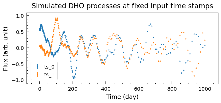
• At fixed input time stamps (use gpSimByTime)

# randomly draw time stamps from a log distribution
tIn = np.logspace(0, np.log10(1000), 500)

# simulate
SNR = 20
tOut, yOut, yerrOut = gpSimByTime(dho_kernel, SNR, tIn, nLC=nLC, log_flux=False)

# plot the simulated process
fig, ax = plt.subplots(1,1, dpi=120, figsize=(8,3))

for i in range(nLC):
    ax.errorbar(tOut[i], yOut[i], yerrOut[i], fmt='.', label=f'ts_{i}', markersize=3)

ax.set_xlabel('Time (day)')
ax.set_ylabel('Flux (arb. unit)')
ax.set_title('Simulated DHO processes at fixed time stamps')
ax.legend(markerscale=1, loc=3)

<matplotlib.legend.Legend at 0x7f87a05fc280>

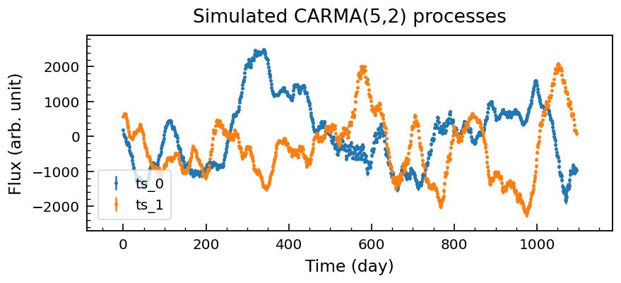
Simulate a CARMA(5,2) process

• At uniformly-spaced time stamps (use gpSimFull)

# define a CARMA(5,2) kernel
ARpars = [6.39255585e-01, 8.19334579e-01, 4.74749350e-01,
          4.08631157e-02, 7.22707479e-04]
MApars = [7.04646183, 0.10365114, 0.79552856]
carma_kernel = CARMA_term(np.log(ARpars), np.log(MApars))

# simulate two time series
nLC = 2
SNR = 20
duration = 365*3.0
npts = 1000
t, y, yerr = gpSimFull(carma_kernel, SNR, duration, npts, nLC=nLC, log_flux=False)

print(f'The number returned time series: {y.shape[0]}')

The number returned time series: 2

# plot the simulated process
fig, ax = plt.subplots(1,1, dpi=120, figsize=(8,3))

for i in range(nLC):
    ax.errorbar(t[i], y[i], yerr[i], fmt='.', label=f'ts_{i}', markersize=4)

ax.set_xlabel('Time (day)')
ax.set_ylabel('Flux (arb. unit)')
ax.set_title('Simulated CARMA(5,2) processes')
ax.legend(markerscale=1, loc=3)

<matplotlib.legend.Legend at 0x7f87a04f18b0>

• At fixed input time stamps (use gpSimByTime)

# randomly draw time stamps from a log distribution
tIn = np.logspace(0, np.log10(2000), 500)

# simulate
SNR = 20
tOut, yOut, yerrOut = gpSimByTime(carma_kernel, SNR, tIn, nLC=nLC, log_flux=False)

# plot the simulated process
fig, ax = plt.subplots(1,1, dpi=120, figsize=(8,3))

for i in range(nLC):
    ax.errorbar(tOut[i], yOut[i], yerrOut[i], fmt='.', label=f'ts_{i}', markersize=3)

ax.set_xlabel('Time (day)')
ax.set_ylabel('Flux (arb. unit)')
ax.set_title('Simulated CARMA(5,2) processes at fixed time stamps')
ax.legend(markerscale=1)

<matplotlib.legend.Legend at 0x7f879ff66c70>

Note

For very high-order models (large p and q), extremely high cadence (> 1000 data points/unit time) may introduce numerical instabilities at solving the autocovariance matrix within \(\mathit{celerite}\), which means that an error will be thrown. One suggested walk around is changing the time unit in your CARMA parameters (e.g., from day to hour).

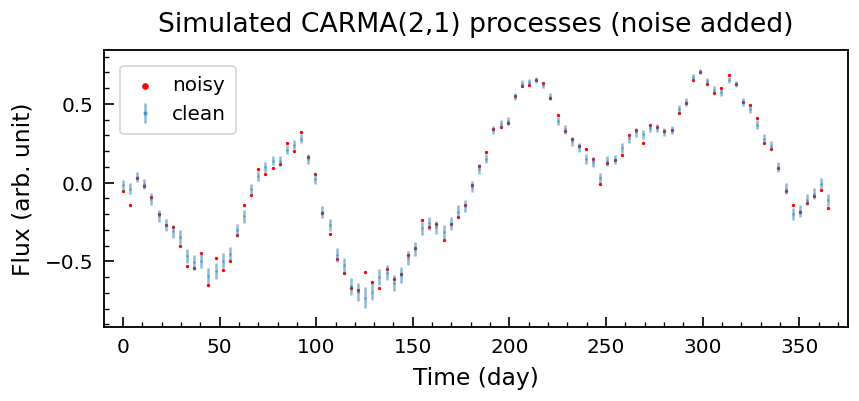
Add noise to a simulated CARMA(2,1) process

• use addNoise

# define a DHO/CARMA(2,1) kernel
dho_kernel = DHO_term(np.log(0.04), np.log(0.0027941), np.log(0.004672),
                      np.log(0.0257))

# simulate a CARMA(2,1) time series
nLC = 1
SNR = 10
duration = 365
npts = 100
t, y, yerr = gpSimFull(dho_kernel, SNR, duration, npts, nLC=nLC, log_flux=False)

# add noise
noisy_y = addNoise(y, yerr)

# overplot the noisy data on top of the 'clean' data
# plot the simulated process
fig, ax = plt.subplots(1,1, dpi=120, figsize=(8,3))

ax.errorbar(t, y, yerr, fmt='.', markersize=1, alpha=0.5, label='clean')
ax.scatter(t, noisy_y, s=1, label='noisy', color='red')
ax.set_xlabel('Time (day)')
ax.set_ylabel('Flux (arb. unit)')
ax.set_title('Simulated CARMA(2,1) processes (noise added)')
ax.set_xlim(0-10, duration+10)
ax.legend()

<matplotlib.legend.Legend at 0x7f8790797cd0>